What is R?
R was created by Rob Gentleman and Ross Ihaka in 1994; it is based on the S language developed at Bell Labs by John Chambers (Stanford Statistics).
It is an open-source language and environment for statistical computing and graphics.
- R offers:
- A simple and effective programming language.
- A data handling and storage facility.
- A suite of libraries for matrix computations.
- A large collection of tools for data analysis.
- Facilities for generating high-quality graphics and data display.
- R is highly extensible, but remains a fully planned and coherent system, rather than an incremental accumulation of specific and inflexible tools.
Who uses R?
Traditionally, academics and researchers. However, recently R has expanded also to industry and enterprise market. Worldwide usage on log-scale:
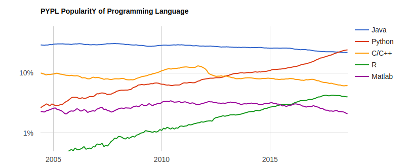
Source: http://pypl.github.io/PYPL.html
The PYPL Index is created by analyzing how often language tutorials are searched on Google (generated using raw data from Google Trends).
Why should you learn R?
Pros:
- Open source and cross-platform.
- Created with statistics and data in mind; new ideas and methods in statistics usually appear in R first.
- Provides a wide range of high-quality packages for data analysis and visualization.
- Arguably, the most commonly used language by data scientists
Cons:
- Performance/Scalability: low speed, poor memory management.
- Some packages are low-quality and provide no support.
- A unconventional syntax and a few unusual features compared to other languages.
A few alternatives to R:
- Python: fastest growing, general-purpose programming, with data science libraries.
- SAS: used for statistical analysis; commercial and expensive, slower development.
- SQL: designed for managing data held in a relational database management system.
- MATLAB: proprietary, mostly for numerical computing, and matrix computations.
What makes R good?
R is an interpreted language, i.e. programs do not need to be compiled into machine-language instructions.
R is object oriented, i.e. it can be extended to include non-standard data structures (objects). A generic function can act differently depending on what objects you passe to it.
R supports matrix arithmetics.
R packages can generate publication-quality plots, and interactive graphics.
Many user-created R packages contain implementations of cutting edge statistics methods.
“Textbook”
We will use R for Data Science as a primary reference. Other resources are listed on the website/
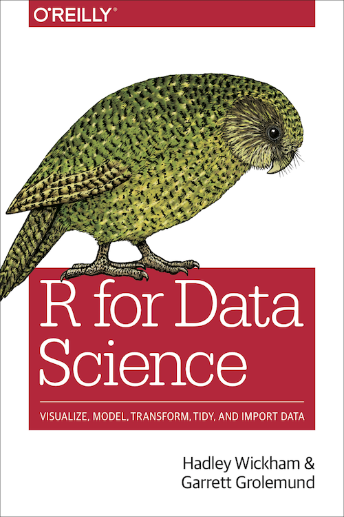
Freely available at: http://r4ds.had.co.nz/
Other useful resources for learning R
Setting up an R environment
Installing R
R is open sources and cross platform (Linux, Mac, Windows).
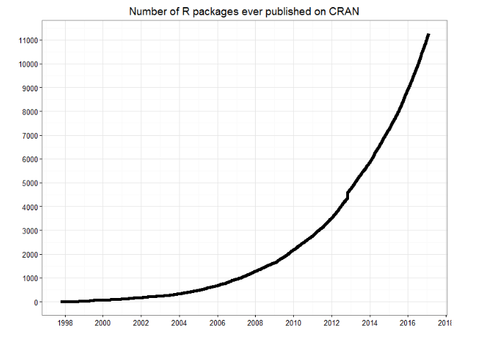
To download it, go to the Comprehensive R Archive Network CRAN website. Download the latest version for your OS and follow the instructions.
Each year a new version of R is available, and 2-3 minor releases. You should update your software regularly.
Running R code
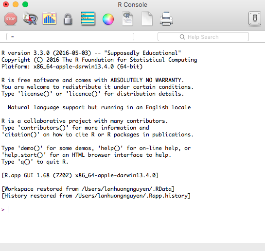
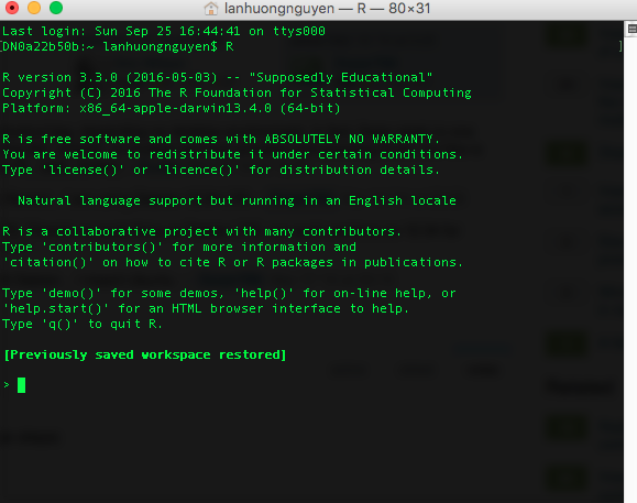
Interpreter mode:
open a terminal and launch R by calling “R” (or open an R console).
type R commands interactively in the command line, pressing Enter to execute.
use q() to quit R.
Scripting mode:
write a text file containing all commands you want to run
save your script as an R script file (e.g. “myscript.R”)
execute your code from the terminal by calling “Rscript myscript.R”
R editors
The most popular R editors are:
- Rstudio, an integrated development environment (IDE) for R.
- Emacs, a free, powerful, customizable editor for many languages.
In this class, we will use RStudio, as it is more user-friendly.
Installing RStudio
RStudio is open-source and cross-platform (Linux, Mac, Windows).
Download and install the latest version for your OS from the official website.
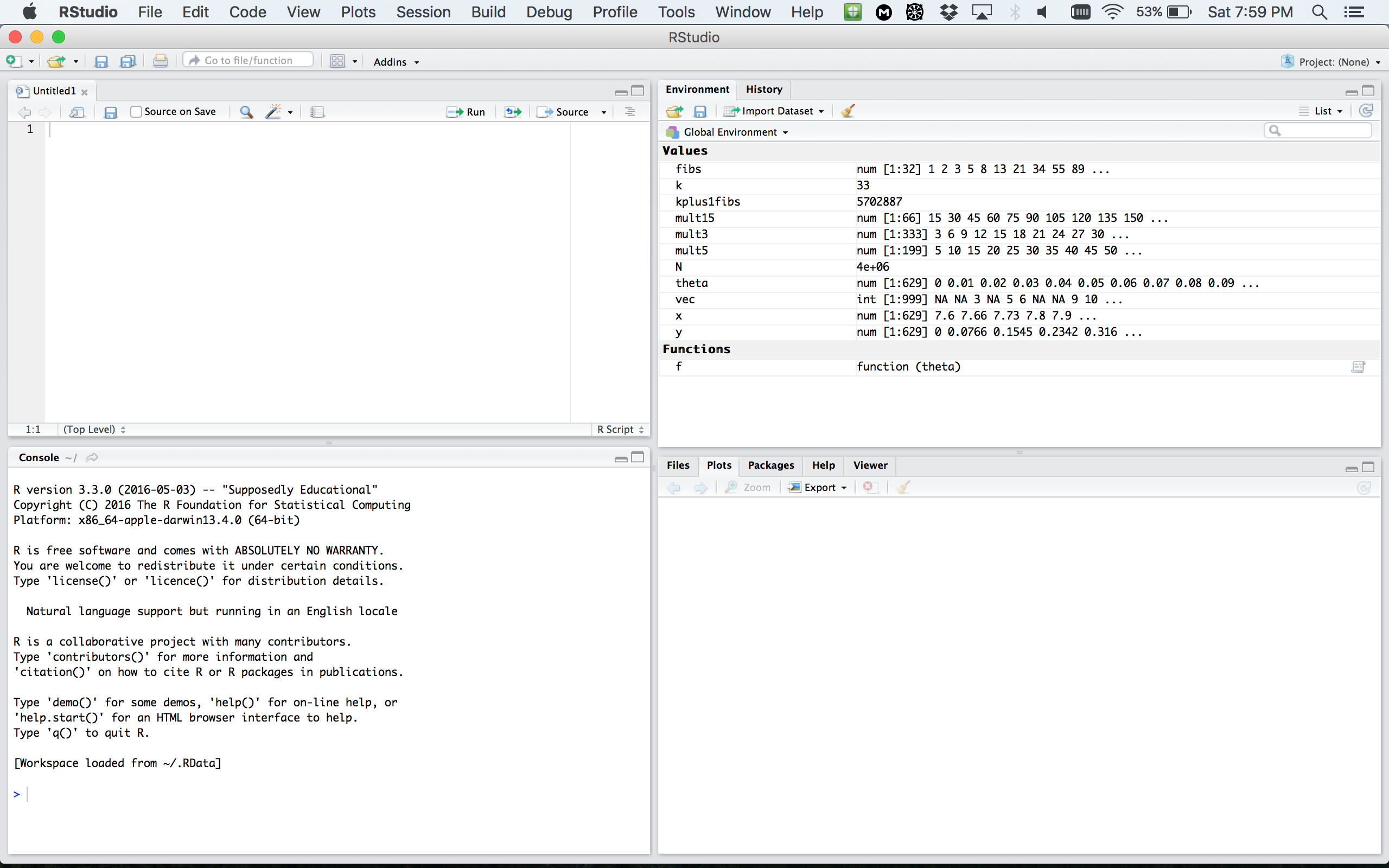
RStudio window
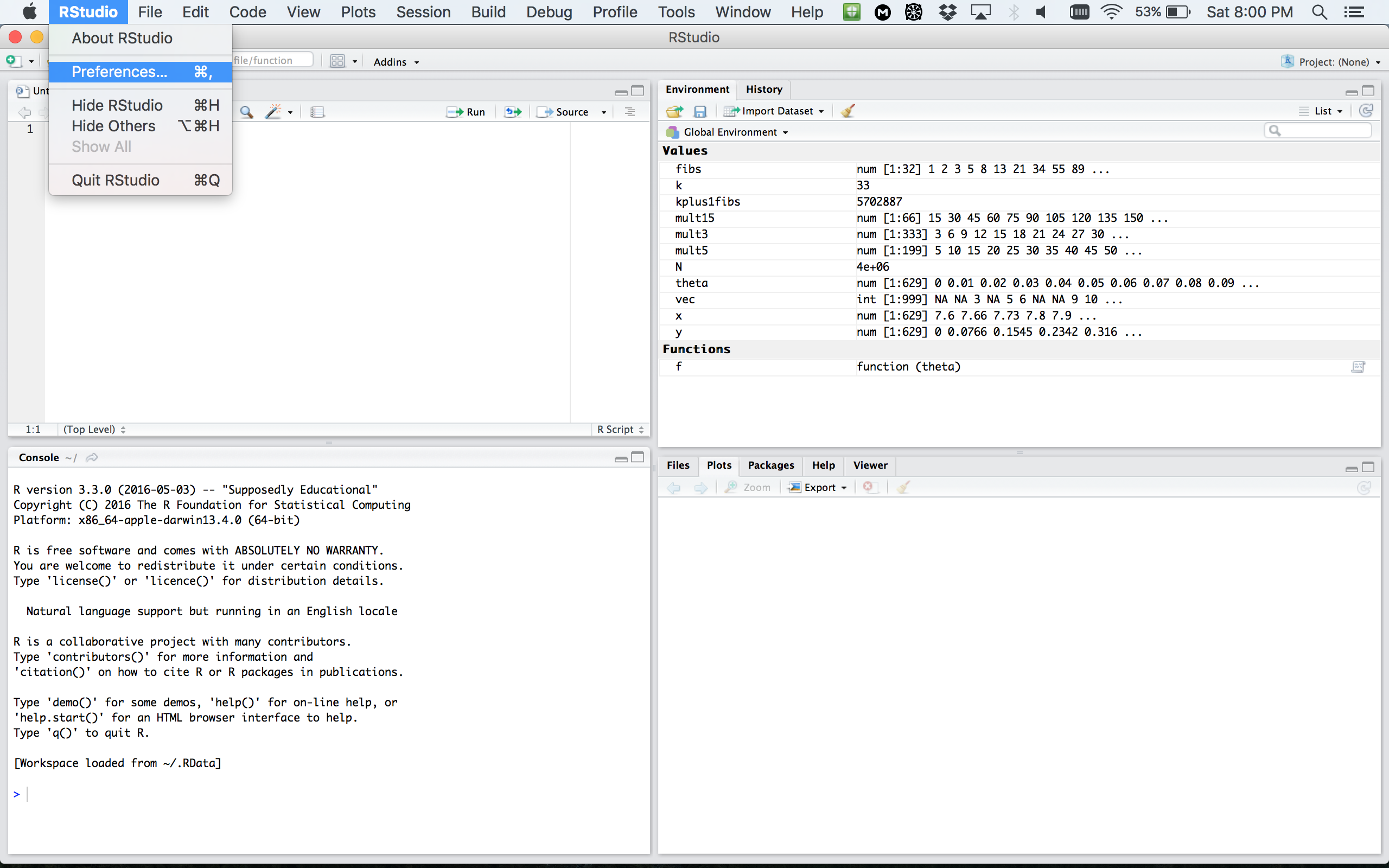
RStudio preferences
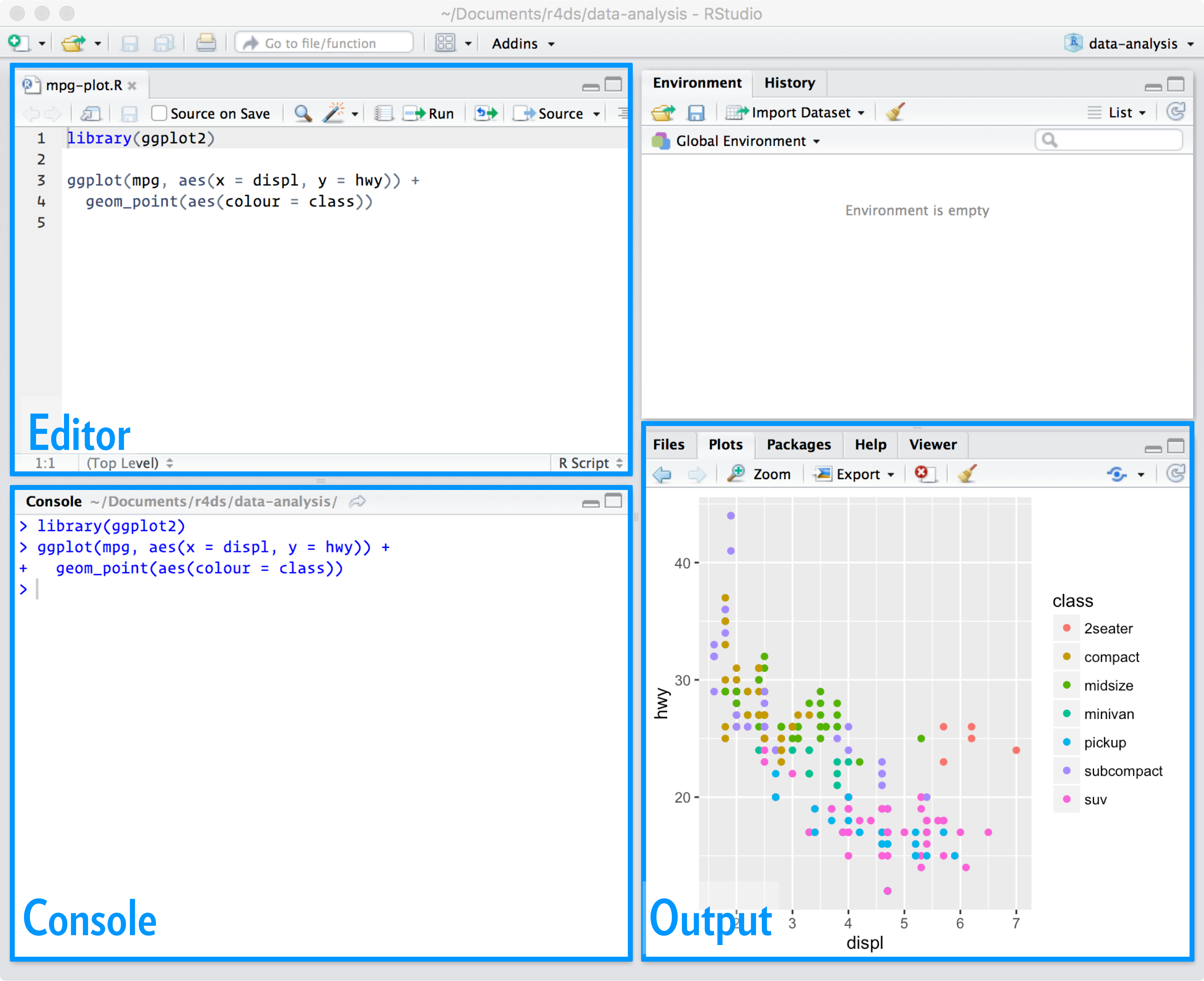
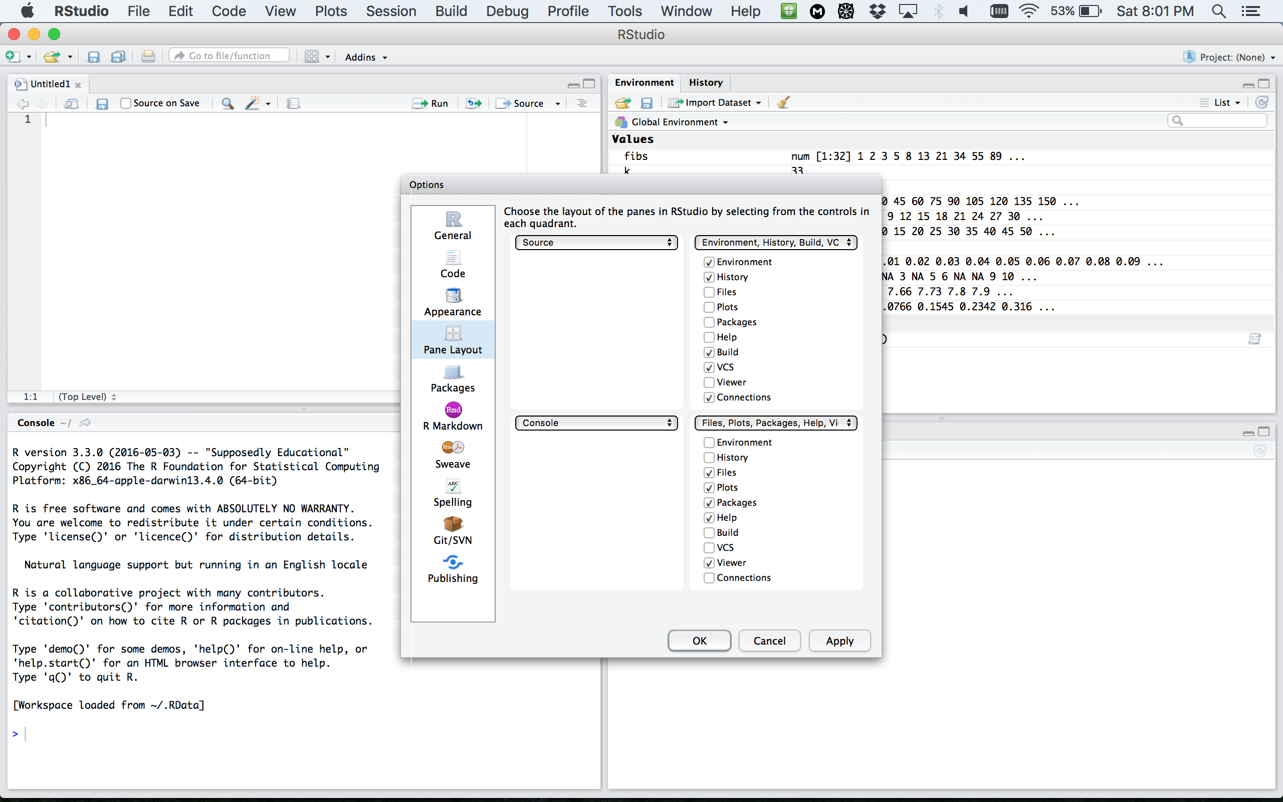
RStudio layout
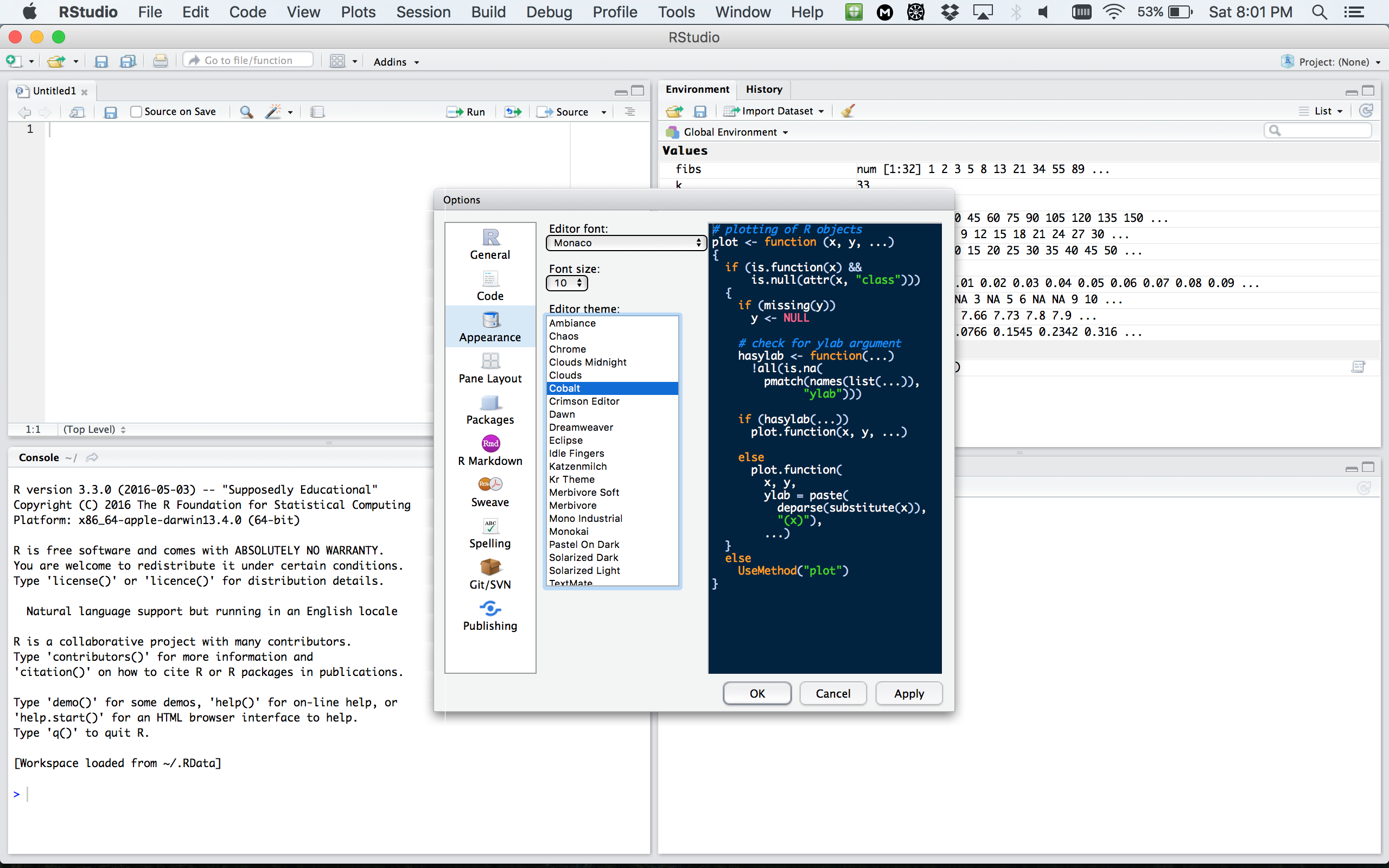
RStudio apprearance
More on RStudio cuztomization can be found here
R document types
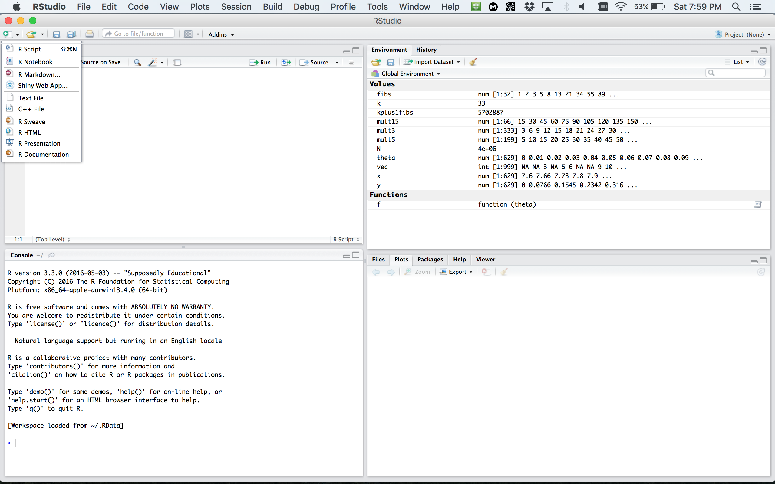
R document types
R Script a text file containing R commands stored together.
R Markdown files can generate high quality reports contatining notes, code and code outputs. Python and bash code can also be executed.
R Notebook is an R Markdown document with chunks that can be executed independently and interactively, with output visible immediately beneath the input.
R presentation let’s you author slides that make use of R code and LaTeX equations as straightforward as possible.
R Sweave enables the embedding of R code within LaTeX documents.
Other documents
R packages
R packages are a collection of R functions, complied code and sample data.
They are stored under a directory called library in the R environment.
Some packages are installed by default during R installation and are always automatically loaded at the beginning of an R session.
- Additional packages by the user from:
- CRAN The first and biggest R repository.
- Bioconductor: Bioinformatics packages for the analysis of biological data.
- github: packages under development
Installing R packages from different repositories:
# install.packages("Package Name"), e.g.
install.packages("glmnet")
# First, load Bioconductor script. You need to have an R version >=3.3.0.
source("https://bioconductor.org/biocLite.R")

# Then you can install packages with:  biocLite("Package Name"), e.g.
biocLite("limma")
# You need to first install a package "devtools" from CRAN
install.packages("devtools")

# Load the "devtools" package
library(devtools)

# Then you can install a package from some user's reporsitory, e.g.
install_github("twitter/AnomalyDetection")

# or using install_git("url"), e.g.
install_git("https://github.com/twitter/AnomalyDetection")
Where are R packages stored?
# Get library locations containing R packages
.libPaths()
## [1] "/Library/Frameworks/R.framework/Versions/3.6/Resources/library"
# Get the info on all the packages installed
installed.packages()[1:5, 1:3]
##                  Package            LibPath                                                          Version
## abind            "abind"            "/Library/Frameworks/R.framework/Versions/3.6/Resources/library" "1.4-5"
## ade4             "ade4"             "/Library/Frameworks/R.framework/Versions/3.6/Resources/library" "1.7-15"
## animation        "animation"        "/Library/Frameworks/R.framework/Versions/3.6/Resources/library" "2.6"
## AnnotationDbi    "AnnotationDbi"    "/Library/Frameworks/R.framework/Versions/3.6/Resources/library" "1.48.0"
## AnnotationFilter "AnnotationFilter" "/Library/Frameworks/R.framework/Versions/3.6/Resources/library" "1.10.0"
# Get all packages currently loaded in the R environment
search()
## [1] ".GlobalEnv" "package:stats" "package:graphics" "package:grDevices" "package:utils" "package:datasets" "package:methods" "Autoloads" "package:base"
Getting you ready for Lab 2
The swirl R package allows to learn R programming and data science very easily. You will use it in Lab 2, so here we are going to install it together. The workflow is the same as for any other R package.
Step 1: Open RStudio and type the following into the console:
install.packages("swirl")
That is just for this time!!! Once swirl is installed on your machine, you can skip directly to step 2.
Step 2: Start swirl
This is the only step that you will repeat every time you want to run swirl. First, you will load the package using the library() function. Then you will call the function that starts the magic! Type the following, pressing Enter after each line:
Getting you ready for Lab 2
The first time you start swirl, you’ll be prompted to install a course. For Lab 2, we’ll ask you to go through a couple of recommended courses. See website for more information.